
M. M. Holland1, M. Bushuk2, A. Jahn3, and A. Roberts4
1Climate and Global Dynamics Laboratory, National Center for Atmospheric Research, Boulder, CO, USA
2Geophysical Fluid Dynamics Laboratory, NOAA, Princeton, NJ, USA
3Department of Atmospheric and Oceanic Sciences and Institute of Arctic and Alpine Research, University of Colorado, Boulder, CO, USA
4Theoretical Division, Los Alamos National Laboratory, Los Alamos, NM, USA
Highlights
- Recent advances, including the use of large model ensembles, satellite simulators for remotely-sensed data comparisons, and data assimilation techniques, have enabled more informative use of Arctic observations for climate simulation assessment, improvements in models, and better forecast initialization.
- These advances in integrating models and observations have increased the skill and utility of Arctic sea ice predictions across timescales from seasons to centuries.
Introduction
The Arctic is rapidly changing in response to rising greenhouse gas concentrations. To better prepare for Arctic change, reliable predictions are needed across a range of timescales. This includes sub-seasonal forecasts that aid near-term planning to multi-decadal projections that allow for informed decisions on climate change mitigation and adaptation. The sources of predictability differ across timescales. Accurate initial conditions are critical for near-term forecasts while longer-term climate projections are subject to assumptions on future climate drivers, such as changing greenhouse gas emissions. These predictions use physics-based models to represent the atmosphere, ocean, sea ice, and land. These models simulate the evolution of environmental conditions on timescales of hours to centuries, and have skillfully predicted Arctic change. Innovative methods for simulation assessment, model development, and forecast initialization are allowing better integration of models and observations to advance predictions.
Using observations to assess climate simulations
Comparison of simulated climate with observations can identify model deficiencies, which may influence the reliability of climate predictions. However, making appropriate comparisons is fraught with challenges. Arctic in situ measurements are sparse and represent single locations instead of the aggregate spatial quantities represented in a model. Remotely sensed data have spatial sampling more comparable to models, albeit often at higher resolution. They rely on algorithms to translate measured signals into environmental properties, which can result in incompatible definitions between remotely sensed and simulated variables. Most observational records are short, typically a few decades or less, and subsurface measurements (e.g., under sea ice) are particularly limited.
A number of new approaches are enabling better use of observations for assessing simulation of Arctic climate. Climate models simulate climate variations over time, including variability that occurs both naturally and in response to external drivers like rising greenhouse gas concentrations. However, the naturally occurring variations are chaotic, meaning that while models simulate these variations, their temporal evolution will not match that of the observations. The advent of large ensembles in which many climate simulations are performed with the same external drivers, but with different simulated natural variations (e.g., Deser et al. 2020), allows us to compare the single observed realization within the envelope of simulated climates. This enables a fairer assessment of simulation quality in light of naturally occurring variability (e.g., for sea ice examples, see Swart et al. 2015; Jahn et al. 2016).
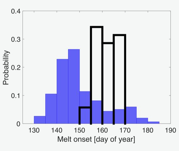
The compilation of remotely-sensed sea ice data beyond ice concentration, such as ice thickness and seasonal indicators (e.g., onset of melt or freeze-up), is enabling more in-depth process-based assessment, which can help identify the cause of model biases. For example, seasonal sea ice change indicators were used in a recent model assessment to reveal that melt onset is simulated too early in many CMIP6 models (Fig. 1; Smith et al. 2020). It also revealed that a bias in melt onset can compensate for a thin ice cover, leading to simulated September extents consistent with observations, but for the wrong physical reasons (Smith et al. 2020). Such process-based model assessments can provide insights on model development needs that can ultimately improve predictions and projections.
Assessment efforts using remotely sensed data have also made advances through the development of satellite simulators within climate models (e.g., Yu et al. 1996). These simulators convert model variables into the remotely sensed measurement quantities, allowing for a direct comparison of the two. Cloud-property simulators (e.g., Bodas-Salcedo et al. 2011) have become widely used and several sea-ice simulators currently under development show promise for better interpreting remotely sensed information for climate modeling (e.g., Burgard et al. 2020a,b).
Using observations to improve models
Measurements are critical for improving the representation of processes within models and are most useful for model development when collated to describe multiple aspects of Arctic phenomena. For this, observations are commonly combined in two distinct ways: First, long records of variables with broad spatial coverage are used to ascertain the likelihood of a simulated state, and its compatibility with observations. Examples of this type of application include quantification of skill and bias of simulated Arctic variability and mean state, for example, for sea ice extent (Yang and Magnusdottir 2018). Second, data of a particular phenomenon are used to characterize its statistical properties for use in model improvements, for example, for sea ice ridging (Roberts et al. 2019). For both of these approaches, sufficiently large datasets are needed that take into account spatial and temporal autocorrelation of the observable quantity, and compatibility between observations and models.
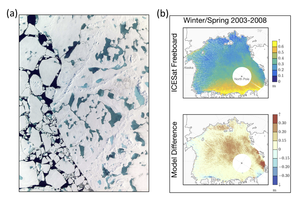
Sea ice has many heterogeneous properties (Fig. 2a) that are important for sea ice melt, growth, and motion, and in turn impact climate. These properties occur at spatial scales below the size of a model grid cell, which is typically around 100 km for a coupled Earth system model, meaning they are not resolved and thus are in need of parameterization. Frequent observations of properties like ice thickness and freeboard, snow conditions, melt-ponds, and mass and energy fluxes over an intensely studied field area are essential for process understanding and for developing statistical aggregations of ridging, snow deposition, albedo, and ponding for use in model parameterizations. However, for some applications, more observations are not always better and autocorrelation and sample size are important when considering the design of an Arctic observing system. For example, simulated ice thickness is highly auto-correlated in space and time (Blanchard-Wrigglesworth and Bitz 2014); therefore, daily freeboard observations within close proximity yield little extra benefit compared to sparser weekly observations when assessing model skill on seasonal to decadal timescales. For this reason, the 91-day repeat orbits of the NASA Ice, Cloud, and land Elevation Satellite—ICESat and ICESat-2 (Markus et al. 2017)—are ideal for evaluating simulations (Fig. 2b), offering broad spatial coverage of the Arctic ice pack, seasonally separated in time, while yielding meaningful compatibility intervals and spatially distributed estimates of ice freeboard as a proxy for thickness. Such evaluations depend on an operational operator (e.g., Bench 2016) for converting modeled ice and snow thickness to satellite-equivalent freeboard.
Using observations for initialized forecasts
The conditions today provide some ability to predict the future state of the system. Initialized forecasts rely on this “initial-value predictability” and thus require an accurate Earth system state as initial conditions. Obtaining this state for the Arctic is challenging given sparse, missing, and uncertain observations. The required accuracy of initial conditions needed to realize skillful forecasts is not clear and differs by variable, the property that is being forecasted (e.g., sea ice area), and the forecast lead time.
Data assimilation (DA) optimally combines observed data to estimate the system state. In recent work, sea ice DA has provided more accurate initial conditions with promise for improving forecasts (e.g., Massonnet et al. 2015). With the recent proliferation of satellite-based ice thickness data, which are important for seasonal ice area predictability (e.g., Day et al. 2014), there are new opportunities to use DA to improve initial conditions (e.g., Blockley and Peterson 2018). Reducing uncertainties in the satellite retrievals and extending them into the ice melt season (i.e., from early spring through the late summer when satellite retrievals of thickness are currently not possible) will allow for more accurate initial conditions, which is expected to substantially improve summer ice forecasts (Bushuk et al. 2020).
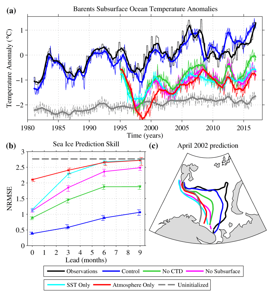
Integrating models with observations can help to quantify the value of existing or proposed observations for prediction. Observing systems experiments (OSEs) assess the influence of existing observations on forecast skill. For example, Bushuk et al. (2019) performed experiments that excluded certain observation types from a global DA system to diagnose the influence on Barents Sea ice predictions. They found that sea surface temperature (SST) observations (see essay Sea Surface Temperature) improved prediction skill on interannual scales, whereas deeper temperature observations improved trend forecasts and corrected the model’s climatological bias (Fig. 3). This work demonstrated the value of ship-based conductivity-temperature-depth (CTD) measurements that are regularly collected in the Barents Sea along with satellite SST observations, emphasizing the need to sustain these crucial observing networks. Observing system simulation experiments (OSSEs) and quantitative network design (e.g., Kaminski et al. 2018) use similar methods to investigate the role of proposed observations for predictions, thereby informing the design of future observing systems.
Taken together, these advances in integrating models and observations have enabled better assessment of Arctic sea ice simulations, the development of improved sea ice models, and improved initialization of sea ice forecasts. This has increased the skill and utility of Arctic sea ice predictions across timescales from seasons to centuries. Collaborations between scientists taking measurements and those developing and utilizing models (e.g., Holland and Perovich 2017) have enabled these advances and will remain critical to continued innovations into the future.
References
Bench, K., 2016: Quantifying seasonal skill in coupled sea ice models using freeboard measurements from spaceborne laser altimeters. Naval Postgraduate School, Monterey, CA. Retrieved from http://hdl.handle.net/10945/49374.
Blanchard-Wrigglesworth, E., and C. M. Bitz, 2014: Characteristics of Arctic sea-ice thickness variability in GCMs. J. Climate, 27(21), 8244-8258.
Blockley, E. W., and K. A. Peterson, 2018: Improving Met Office seasonal predictions of Arctic sea ice using assimilation of CryoSat-2 thickness. Cryosphere, 12, 3419-3438, https://doi.org/10.5194/tc-12-3419-2018.
Bodas-Salcedo, A., and Coauthors, 2011: COSP: Satellite simulation software for model assessment. Bull. Amer. Meteor. Soc., 92, 1023-1043, https://doi.org/10.1175/2011BAMS2856.1.
Burgard, C., D. Notz, L. T. Pedersen, and R.T. Tonboe, 2020a: The Arctic Ocean observation operator for 6.9 GHz (ARC3O)-Part 1: How to obtain sea ice brightness temperatures at 6.9 GHz from climate model output. Cryosphere, 14(7), 2369-2386, https://doi.org/10.5194/tc-14-2369-2020.
Burgard, C., D. Notz, L. T. Pedersen, R. T. Tonboe, 2020b: The Arctic Ocean observation operator for 6.9 GHz (ARC3O)-Part 2: Development and evaluation. Cryosphere, 14, 2387-2407, https://doi.org/10.5194/tc-14-2387-2020.
Bushuk, M., M. Winton, D. B. Bonan, E. Blanchard-Wrigglesworth, and T. Delworth, 2020: A mechanism for the Arctic sea ice spring predictability barrier. Geophys. Res. Lett., 47, e2020GL088335, https://doi.org/10.1029/2020GL088335.
Bushuk, M., X. Yang, M. Winton, R. Msadek, M. Harrison, A. Rosati, and R. Gudgel, 2019: The value of sustained ocean observations for sea ice predictions in the Barents Sea. J. Climate, 32(20), 7017-7035, https://doi.org/10.1175/JCLI-D-19-0179.1.
Day, J. J., E. Hawkins, and S. Tietsche, 2014: Will Arctic sea ice thickness initialization improve seasonal forecast skill? Geophys. Res. Lett., 41, 7566-7575, https://doi.org/10.1002/2014GL061694.
Deser, C., and Coauthors, 2020: Insights from Earth system model initial-condition large ensembles and future prospects. Nat. Climate Change, 10, 277–286, https://doi.org/10.1038/s41558-020-0731-2.
Holland, M. M., and D. Perovich, 2017: Sea ice summer camp: Bringing together sea ice modelers and observers to advance polar science. Bull. Amer. Meteor. Soc., 98(10), 2057-2059, https://doi.org/10.1175/BAMS-D-16-0229.1.
Jahn, A., J. E. Kay, M. M. Holland, and D. M. Hall, 2016: How predictable is the timing of a summer ice-free Arctic? Geophys. Res. Lett., 43, 9113-9120, https://doi.org/10.1002/2016GL070067.
Kaminski, T., and Coauthors, 2018: Arctic mission benefit analysis: impact of sea ice thickness, freeboard, and snow depth products on sea ice forecast performance. Cryosphere, 12, 2569-2594, https://doi.org/10.5194/tc-12-2569-2018.
Markus, T., and Coauthors, 2017: The Ice, Cloud, and land Elevation Satellite-2 (ICESat-2): science requirements, concept, and implementation. Remote Sens. Environ., 190, 260-273, https://doi.org/10.1016/j.rse.2016.12.029.
Massonnet, F., T. Fichefet, and H. Goosse, 2015: Prospects for improved seasonal Arctic sea ice predictions from multivariate data assimilation. Ocean Model., 88, 16-25, https://doi.org/10.1016/j.ocemod.2014.12.013.
Roberts, A. F., E. C. Hunke, S. Kamal, W. F. Lipscomb, C. Horvat, and W. Maslowski, 2019: A variational method for sea ice ridging in Earth System Models. J. Adv. Model. Earth Sys., 11, 771-805, https://doi.org/10.1029/2018MS001395.
Smith, A., A. Jahn, and M. Wang, 2020: Seasonal transition dates can reveal biases in Arctic sea ice simulations. Cryosphere, 14, 2977-2997, https://doi.org/10.5194/tc-14-2977-2020.
Steele, M., A. Bliss, G. Peng, W. N. Meier, and S. Dickinson, 2019: Arctic sea ice seasonal change and melt/freeze climate indicators from satellite data, Version 1, Data subset: 1979-03-01 to 2017-02-28. Data accessed 2019-08-26, 2019.
Swart, N. C., J. C. Fyfe, E. Hawkins, J. E. Kay, and A. Jahn, 2015: Influence of internal variability on Arctic sea-ice trends. Nat. Climate Change, 5, 86-89, https://doi.org/10.1038/nclimate2483.
Yang, W., and G. Magnusdottir, 2018: Year-to-year variability in Arctic minimum sea ice extent and its preconditions in observations and the CESM Large Ensemble simulations. Sci. Rep., 8(1), 9070, https://doi.org/10.1038/s41598-018-27149-y.
Yu, W., M. Doutriaux, G. Sèze, H. Le Treut, and M. Desbois, 1996: A methodology study of the validation of clouds in GCMs using ISCCP satellite observations. Climate Dyn., 12, 389-401, https://doi.org/10.1007/BF00211685.
November 12, 2020